Attention Mechanism from Scratch
A minimal Rust implementation demonstrating how scaled dot-product attention works. -> https://github.com/Shreyas220/llm-playground/tree/main/attention-playground
What is Attention?
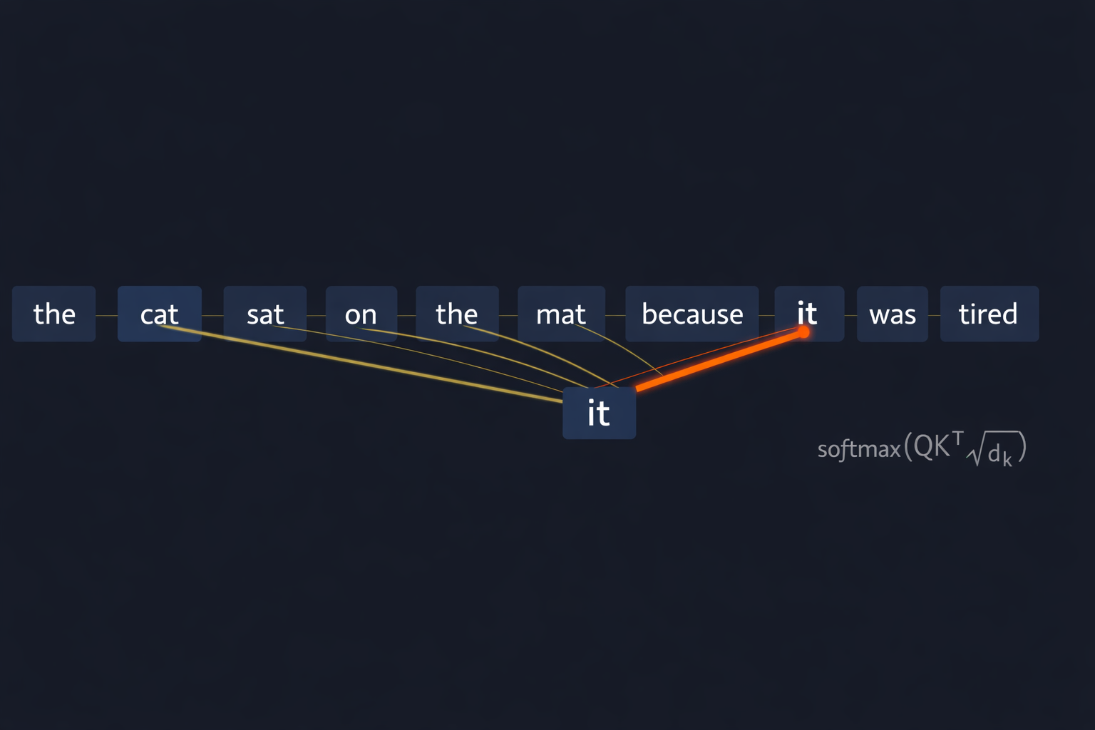
Imagine reading the sentence: “The cat sat on the mat because it was tired.”
What does “it” refer to?
I would instinctively look back at “cat” and that is called attention.
Our brain assigns relevance in some way assigned scores to previous words cat when processing the current it.
Attention mechanisms let neural networks do the same thing, focus on relevant parts of the input.
Now my goal is to understand how this relevance is assigned mathematically. We will start small
The Core Idea
Every attention layer asks a question: “Which other tokens should I pay attention to?”
To answer this, each token gets three vectors:
Think of this like a database lookup:
- Query (Q): The search term you type (e.g., “tired entity”).
- Key (K): The labels or metadata on the database records (e.g., “cat: living”, “mat: object”).
- Value (V): The actual data inside the record you want to retrieve.
In a standard Hash Map, you look for an exact match ($Key == Query$). In Attention, we look for a similarity match ($Key \approx Query$).
Attention score = how well a Query matches a Key.
The Math, Step by Step
Step 1: Computing Similarity with Dot Product
The dot product measures how “aligned” two vectors are:
Q = [2, 3]      ← Query: "what I'm looking for"

Keys:
  C = [11, 13]  ← Key C
  A = [1,  2]   ← Key A
  B = [4,  6]   ← Key B
Computing Q · each Key:
Q · C = 2×11 + 3×13 = 22 + 39 = 61  ← High similarity!
Q · A = 2×1  + 3×2  = 2  + 6  = 8   ← Low similarity
Q · B = 2×4  + 3×6  = 8  + 18 = 26  ← Medium similarity

Scores = [61, 8, 26]
Intuition: The dot product is large when vectors point in similar directions. Q and C are most aligned, so C gets the highest score.
Step 2: Converting Scores to Probabilities (Softmax)
Raw scores can be any number. We need probabilities that sum to 1:
softmax(xᵢ) = eˣⁱ / Σeˣʲ
For scores [61, 8, 26]:
e⁶¹ ≈ 10²⁶    (huge!)
e⁸  ≈ 2981
e²⁶ ≈ 10¹¹

softmax ≈ [≈1.0, ≈0.0, ≈0.0]
Problem: The exponential makes large differences extreme. Token C gets ALL the attention, A and B get essentially zero.
Step 3: Why We Need Scaling for the dot product
Here’s the critical insight from the original “Attention Is All You Need” paper.
Consider high-dimensional vectors with 100 dimensions
dₖ = 100 dimensions

q  = [1, 1, 1, 1, ... 1]      ← 100 ones
K₁ = [1, 1, 1, 1, ... 1]      ← Perfect match
K₂ = [0.8, 0.8, 0.8, ... 0.8] ← Pretty good match (80% similar)
Without scaling:
Q · K₁ = 1×1 + 1×1 + ... (100 times) = 100
Q · K₂ = 1×0.8 + 1×0.8 + ... (100 times) = 80

Difference = 20 points
Now softmax:
softmax([100, 80]) = [e¹⁰⁰, e⁸⁰] / (e¹⁰⁰ + e⁸⁰)
                    ≈ [1.0, 0.0]
The model is overconfident! It says K₁ gets 100% attention and K₂ gets 0%, even though K₂ was 80% similar.
Why this happens: In high dimensions, dot products naturally have larger magnitudes. The variance of a dot product grows with dimension d. This pushes softmax into saturation where gradients vanish.
The fix —> scale by 1/√dₖ:
1/√dₖ (Scaling): We divide by the square root of the dimension to prevent the dot products from exploding.
scaled_scores = [100, 80] / √100 = [10, 8]

softmax([10, 8]) = [e¹⁰, e⁸] / (e¹⁰ + e⁸)
                  ≈ [0.88, 0.12]
Now K₂ gets 12% of attention, the model acknowledges uncertainty!
The scaling factor 1/√dₖ normalizes variance, keeping softmax in a healthy range regardless of embedding dimension.
Step 4: Weighted Sum of Values
Once we have attention weights, we compute a weighted average of Value vectors:
weights = [0.88, 0.12]
V₁ = [...]  ← Value vector for K₁
V₂ = [...]  ← Value vector for K₂

output = 0.88 × V₁ + 0.12 × V₂
The Complete Formula
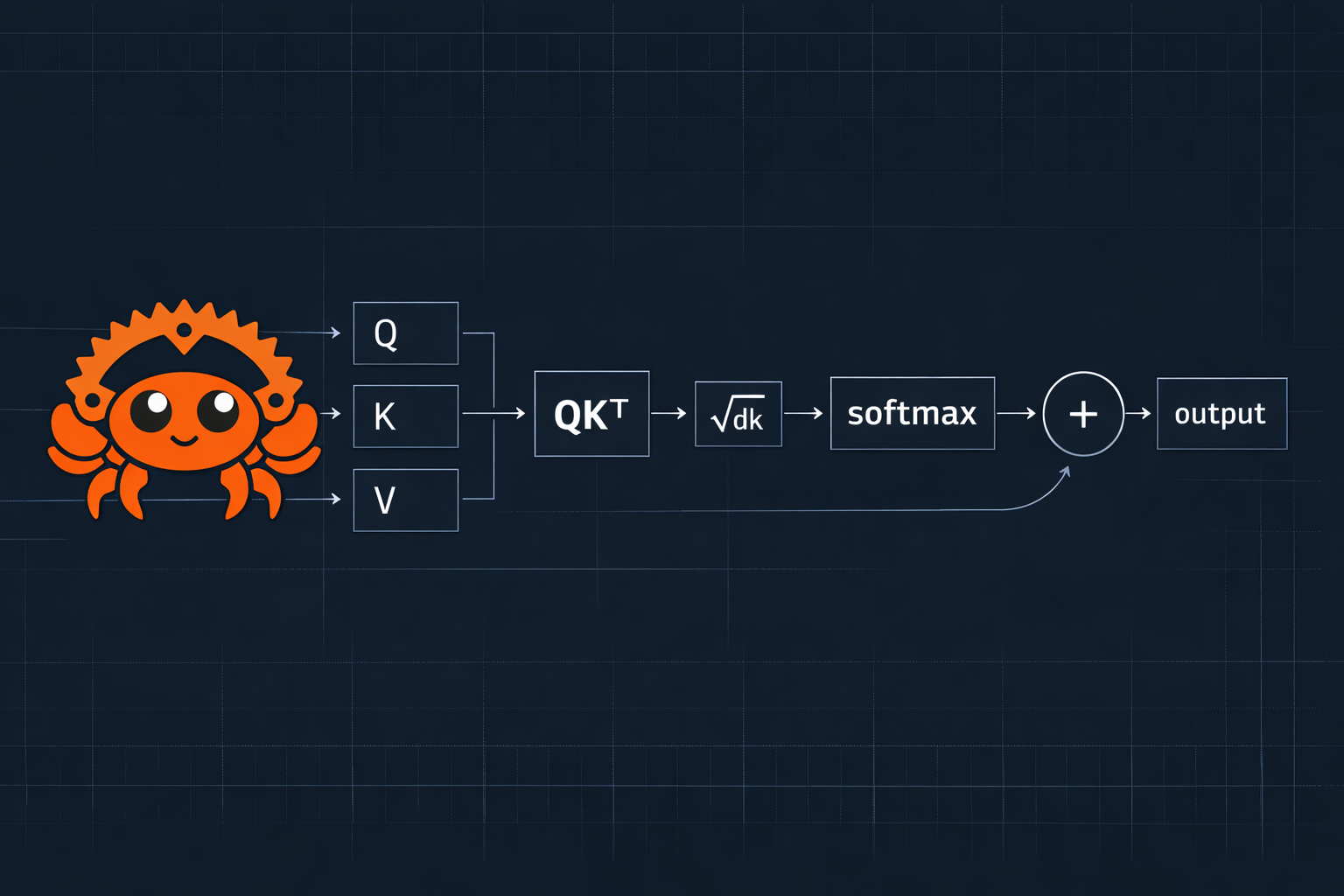
Attention(Q, K, V) = softmax(QKᵀ / √dₖ) · V
Where:
QKᵀcomputes all pairwise similarities√dₖprevents softmax saturation (dₖ = dimension of keys)softmaxconverts to probabilities· Vblends values by those probabilities
In multi-head attention: dₖ = dₘₒₐₑₗ / h (model dimension / number of heads)
From Simple Similarity to True Understanding
What Our POC Does: Semantic Similarity
Our implementation uses raw GloVe embeddings, pre-trained vectors that capture word co-occurrence patterns.
"The king and queen ruled the kingdom"

kingdom → king:   29.5%  ████████   ✓ Works!
kingdom → queen:  18.3%  █████      ✓ Works!
queen → king:     39.5%  ██████████ ✓ Works!
Why it works: GloVe learned that “king”, “queen”, and “kingdom” appear in similar contexts (royalty, monarchy, medieval). Their vectors point in similar directions, so dot product is high.
What Our POC Can’t Do: Coreference
Remember our opening example? Let’s try it:
"The cat sat on the mat because it was tired"

it → cat:      3.7%   █         ✗ Fails!
it → because:  22.8%  ██████    ✗ Wrong!
it → mat:      0.9%   ░
Why it fails: “it” and “cat” don’t appear in similar contexts in text. GloVe has no idea that “it” refers to “cat” in this sentence. That requires understanding grammar, not just word similarity.
The Gap: Similarity vs. Relationship
| Task | Example | Raw Embeddings | Needs Training |
|---|---|---|---|
| Semantic similarity | king ↔ queen | ✅ Works | No |
| Verb-object | ruled → kingdom | ✅ Partial | Better with training |
| Coreference | it → cat | ❌ Fails | Yes |
| Negation | “not happy” means sad | ❌ Fails | Yes |
How Attention Enables Context Understanding
This is where learnable projection matrices (W_Q, W_K, W_V) become crucial.
Raw Embeddings (Our POC)
embed("it")  = [0.2, -0.1, 0.4, ...]   → used directly as Query
embed("cat") = [0.8, 0.3, -0.2, ...]   → used directly as Key

Query · Key = low (vectors aren't aligned)
Learned Projections (Real Transformers)
embed("it")  × W_Q = Query  →  "I'm a pronoun looking for my referent"
embed("cat") × W_K = Key    →  "I'm an animate noun that could be tired"

Query · Key = HIGH (projections learned to align these!)
The magic: W_Q and W_K are learned during training on millions of examples where the model had to figure out what “it” refers to. Through backpropagation, these matrices adjust so that:
- Pronouns’ Queries align with their referents’ Keys
- Verbs’ Queries align with their subjects/objects’ Keys
- Adjectives’ Queries align with the nouns they modify
Running the Code
clone the repo https://github.com/Shreyas220/llm-playground/tree/main/attention-playground
Download GloVe Embeddings
First, download the pre-trained GloVe embeddings:
cd attention-playground
curl -L -o data/glove.6B.zip https://nlp.stanford.edu/data/glove.6B.zip
unzip data/glove.6B.zip -d data/ glove.6B.50d.txt
rm data/glove.6B.zip
Run the Program
# Analyze a sentence
cargo run -- "The king and queen ruled the kingdom"

# Disable self-attention (tokens can't attend to themselves)
cargo run -- --no-self "The king and queen ruled the kingdom"
Example Output
Token 'king' attending to sequence:

  Attention weights for 'king':
    the          0.0647  █
    king         0.4431  █████████████
    and          0.0489  █
    queen        0.1645  ████
    ruled        0.0629  █
    the          0.0647  █
    kingdom      0.1512  ████
Notice “king” attends most to itself (44%), but also finds “queen” (16%) and “kingdom” (15%) — the semantically related words.
Key Takeaways
| Concept | Why It Matters |
|---|---|
| Dot Product | Measures vector alignment — similar meanings → higher scores |
| Scaling (1/√dₖ) | Prevents overconfidence in high dimensions |
| Softmax | Turns scores into a probability distribution |
| Weighted Sum | Blends information based on relevance |
The 1/√dₖ scaling factor is subtle but crucial.
It’s the difference between a model that learns nuanced relationships and one that makes overconfident binary decisions.
References
- Attention Is All You Need — The original transformer paper
- GloVe: Global Vectors for Word Representation
- Attention: 3Blue1Brown video